Unique Games and Small Set Expansion
The Unique Games Conjecture (UGC) (Khot 2002) states that for every \(\epsilon>0\) there is some finite \(\Sigma\) such that the \(1-\epsilon\) vs. \(\epsilon\) problem for the unique games problem with alphabet \(\Sigma\) is NP hard. An instance to this problem can be viewed as a set of equations on variables \(x_1,\ldots,x_n \in \Sigma\) where each equation has the form \(x_i = \pi_{i,j}(x_j)\) where \(\pi_{i,j}\) is a permutation over \(\Sigma\).
The order of quantifiers here is crucial. Clearly there is a propagation type algorithm that can find a perfectly satisfying assignment if one exist, and as we mentioned before, it turns out that there is also an algorithm nearly satisfying assignment (e.g., satisfying \(0.99\) fraction of constraints) if \(\epsilon\) tends to zero independently of \(\Sigma\). However, when the order is changed, the simple propagation type algorithms fail. That is, if we guess an assignment to the variable \(x_1\), and use the permutation constraints to propagate this guess to an assignment to \(x_1\)’s neighbors and so on, then once we take more than \(O(1/\epsilon)\) steps we are virtually guaranteed to make a mistake, in which case our propagated values are essentially meaningless. One way to view the unique games conjecture is as stating this situation is inherent, and there is no way for us to patch up the local pairwise correlations that the constraints induce into a global picture. While the jury is still out on whether the conjecture is true as originally stated, we will see that the sos algorithm allows us in some circumstances to do just that. The small set expansion (SSE) problem (Raghavendra and Steurer 2010) turned out to be a clean abstraction that seems to capture the “combinatorial heart” of the unique games problem, and has been helpful in both designing algorithms for unique games as well as constructing candidate hard instances for it. We now describe the SSE problem and outline the known relations between it and the unique games problem.
For every undirected \(d\)-regular graph \(G=(V,E)\), and \(\delta>0\) the expansion profile of \(G\) at \(\delta\) is \[ \varphi_\delta(G) = \min_{S\subseteq V , |S|\leq \delta |V|} |E(S,\overline{S})|/(d|S|) \;. \] For \(0 < c < s <1\), the \(c\) vs \(s\) \(\delta\)-SSE problem is to distinguish, given a regular undirected graph \(G\), between the case that \(varphi_\delta(G) \leq c\) and the case that \(\varphi_\delta(G) \geq s\).
The small set expansion hypothesis (SSEH) is that for every \(\epsilon>0\) there is some \(\delta\) such that the \(\epsilon\) vs \(1-\epsilon\) \(\delta\)-SSE problem is NP hard.
We will see that every instance of unique games on alphabet \(\Sigma\) gives rise naturally to an instance of \(\tfrac{1}{|\Sigma|}\)-SSE. But the value of the resulting instance is not always the same as the original one, and hence this natural mapping does not yield a valid reduction from the unique games to the SSE problem. Indeed, no such reduction is known. However, Raghavendra and Steurer (2010) gave a highly non trivial reduction in the other direction (i.e., reducing SSE to UG) hance showing that the SSEH implies the UGC. Hence, assuming the SSEH yields all the hardness results that are known from the UGC, and there are also some other problems such as sparsest cut where we only know how to establish hardness based on the SSEH and not the UGC (Raghavendra, Steurer, and Tulsiani 2012).
Embedding unique games into small set expansion
Given a unique games instance \(I\) on \(n\) variables and alphabet \(\Sigma\), we can construct a graph \(G(I)\) (known as the label extended graph corresponding to \(I\)) on \(n|\Sigma|\) vertices where for every equation of the form \(x_i = \pi_{i,j}(x_j)\) we connect the vertex \((i,\sigma)\) with \((j,\tau)\) if \(\pi_{i,j}(\tau)=\sigma\). Note that every assignment \(x\in\Sigma^n\) is naturally mapped into a subset \(S\) of size \(n\) (i.e. \(1/|\Sigma|\) fraction) of the vertices of \(G(I)\) corresponding to the vertices \(\{ (i,x_i) : i\in [n] \}\). Let’s assume for simplicity that in the unique games instance every variable participated in exactly \(d\) of the constraints (and hence there is a total of \(nd/2\) constraints). Then the graph \(G\) will have degree \(d\) and every constraint \(x_i \neq \pi_{i,j}(x_j)\) that is violated by \(x\) contributes exactly two edges to \(E(S,\overline{S})\) (the edges \(\{ (i,x_i),(j,\pi_{i,j}^{-1}(x_i))\}\) and \(\{ (i,\pi_{i,j}(x_j)),(j,x_j)\}\)). Hence the fraction of violated constraints by \(x\) is equal to \(E(S,\overline{S})/(d|S|)\).
However, this is not a valid reduction, since we cannot do this mapping in reverse. That is, the graph \(G\) might have a set \(S\) of \(n\) vertices that does not expand that does not correspond to any assignment for the unique games. It can be shown that this reduction is valid if the constraint graph of the unique games instance is a small set expander in the sense that every set of \(o(1)\) fraction of the vertices has expansion \(1-o(1)\).
The known algorithmic results for small set expansion are identical to the ones known for unique games:
- The basic SDP algorithm can solve the \(1-\epsilon\) vs \(1-O(\sqrt{\epsilon\log(1/\delta)})\) \(\delta\)-SSE problem (Raghavendra, Steurer, and Tetali 2010) which matches the \(1-\epsilon\) vs \(1-O(\sqrt{\epsilon \log |\Sigma|})\) algorithm for the \(\Sigma\)-UG problem of Charikar, Makarychev, and Makarychev (2006) (which itself generalizes the \(1-\epsilon\) vs \(1-O(\sqrt{\epsilon})\) Goemans and Williamson (1995) for Max Cut).
- When \(\delta \ll \epsilon\) (specially \(\delta < \exp(\Omega(1/\epsilon))\)) then no polynomial time algorithm is known. However, Arora, Barak, and Steurer (2015) showed a \(\exp(\poly(1/\delta)n^{\poly(1/\epsilon)})\) time algorithm for the \(1-\epsilon\) vs \(1/2\) \(\delta\)-SSE problem and similarly a \(\exp(\poly(|\Sigma|)n^{\poly(1/\epsilon)})\) time algorithm for the \(1-\epsilon\) vs \(1/2\) \(\Sigma\)-UG problem.
Thus it is consistent with current knowledge that the \(1-\epsilon\) vs
\(\epsilon\) \(\Sigma\)-UG computational problem has complexity equivalent
(up to polynomial factors) to the \(1-\epsilon\) vs \(\epsilon\)
\(\tfrac{1}{|\Sigma|}\)-SSE problem. At the moment one can think of the
small set expansion problem as the “easiest” “UG like” problem and the
Max-Cut (or Max \(2LIN(2)\)) problem as the “hardest” “UG like” problem
where by “UG like” we mean problems that in the perfect case can be
solved by propagation like algorithms and that we suspect might have a
subexponential time algorithm.
(Such algorithms are known for unique games and small set expansion but
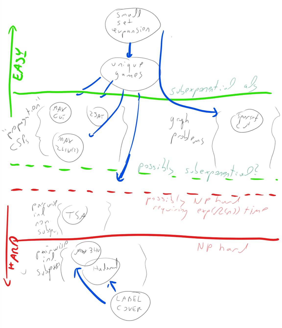
not for Max Cut.) Unique Games itself can be thought of as lying
somewhere between these two problems. The following figure represents
are current (very partial) knowledge of the landscape of complexity for
CSPs and related graph problems such as small set expansion and sparsest
cut
Small set expansion as finding “analytically sparse” vectors.
We have explained that the defining feature of “unique games like” problems is the fact that they exhibit strong pairwise correlations. One way to see it is that these problems have the form of trying to optimize a quadratic polynomial \(x^\top A x\) over some “structured” set \(x\):
- The maximum cut problem can be thought as the task of maximizing \(x^\top L x\) over \(x\in \{ \pm 1 \}^n\) where \(L\) is the Laplacian matrix of the graph.
- The sparsest cut problem can be thought of as the task of minimizing the same polynomial \(x^\top L x\) over unit vectors (in \(\ell_2\) norm) of the form \(x\in\{0,\alpha\}^n\) for some \(\alpha>0\).
- The small set expansion problem can be thought of as the task of minimizing the same polynomial \(x^\top L x\) over unit vectors of the form \(x\in \{0,\alpha\}^n\) subject to the condition that \(\norm{x}_1/\sqrt{n} \leq \sqrt{\delta}\) (which corresponds to the condition that \(\alpha \geq 1/\sqrt{n\delta}\)).
- The unique games problem can be thought of as the task of minimizing the polynomial \(x^\top L x\) where \(L\) is the Laplacian matrix corresponding to the label extended graph of the game and \(x\) ranges over all vectors in \(\zo^{n|\Sigma|}\) such that for every \(i\in [n]\) there exists exactly one \(\sigma\in\Sigma\) such that \(x_{i,\sigma}=1\).
In all of these cases the computational question we are faced with amounts to what kind of global information can we extract about the unknown assignment \(x\) from the the local pairwise information we get by knowing the expected value of \((x_i-x_j)^2\) over an average edge \(i\sim j\) in the graph.
Proxies for sparsity
We see that all these problems amount to optimizing some quadratic polynomial \(q(x)\) over unit vector \(x\)’s that are in some structured set. By “guessing” the optimum value \(\lambda\) that \(q(x)\) can achieve, we can move to a “dual” version of these problems where we want to maximize \(p(x)\) over all \(x\in\R^n\) such that \(q(x)=\lambda\) where \(p(x)\) is some “reward function” that is larger the closer that \(x\) is to our structured set (equivalently, one can look at \(-p(x)\) as a function that penalizes \(x\)’s that are far from our structured set).
In fact, in our setting this \(\lambda\) will often be (close to) the minimum or maximum of \(q(\cdot)\) which means that when \(x\) achieves \(q(x)=\lambda\) then all the directional derivatives of the quadratic \(q\) (which are linear functions) vanish. Another way to say it is that the condition \(q(x)=\lambda\) will correspond to \(x\) being (almost) inside some linear subspace \(V\subseteq \R^n\) (which will be the eigenspace of \(q\), looked at as a matrix, corresponding to the value \(\lambda\) and other nearby values). This means that we can reduce our problem to the task of approximating the value \[ \max_{x\in V, \norm{x}=1} p(x) \label{eq:reward} \] where \(p(\cdot)\) is a problem-specific reward function and \(V\) is a linear subspace of \(\R^n\) that is derived from the input. This formulation does not necessarily make the problem easier as \(p(\cdot)\) can (and will) be a non convex function, but, when \(p\) is a low degree polynomial, it does make it potentially easier to analyze the performance of the sos algorithm. That being said, in none of these cases so far we have found the “right” reward function \(p(\cdot)\) that would yield a tight analysis for the sos algorithm. But for the small set expansion question, there is a particularly natural and simple reward function that shows promise for better analysis, and this is what we will focus on next.
Choosing such a reward function might seem to go against the “sos philosophy” where we are not supposed to use creativity in designing the algorithm, but rather formulate a problem such as small set expansion as an sos program in the most straightforward way, without having to guess a clever reward function. We believe that in the cases we discussed, it is possible to consign the choice of the reward function to the analysis of the standard sos program. That is, if one is able to show that the sos relaxation for \eqref{eq:reward} achieves certain guarantees for the original small set expansion problem, then it should be possible to show that the standard sos program for small set expansion would achieve the same guarantees.
Norm ratios as proxies for sparsity
In the small set expansion we are trying to minimize the quadratic \(x^\top L x\) subject to \(x\in \{0,\alpha\}\) being sparse. It turns out that the sparsity condition is more significant than the Booleanity. For example, we can show the following result:
Suppose that \(x\in \R^n\) has at most \(\delta n\) nonzero coordinates, and satisfies \(x^\top L x \leq \epsilon \norm{x}^2\) where \(L\) is the Laplacian of an \(n\)-vertex \(d\)-regular graph \(G\). Then there exists a set \(S\) of at most \(\delta n\) of \(G\)’s vertices such that \(|E(S,\overline{S})| \leq O(\sqrt{\epsilon} dn)\).
It turns out that this theorem can be proven in much the same way that Cheeger itself is proven, showing that a random level set of \(x\) (chosen such that it will have the support be a subset of the nonzero coordinates of \(x\)) will satisfy the needed condition. Note that if \(x\) has at most \(\delta n\) nonzero coordinates then \(\norm{x}_1 \leq \sqrt{n\delta}\norm{x}_2\). It turns out this condition is sufficient for the above theorem:
Suppose that \(x\in \R^n\) satisfies \(\norm{x}_1 \leq \sqrt{\delta n}\norm{x}_2\), and satisfies \(x^\top L x \leq \epsilon \norm{x}^2\) where \(L\) is the Laplacian of an \(n\)-vertex \(d\)-regular graph \(G\). Then there exists a set \(S\) of at most \(O(\sqrt{\delta} n)\) of \(G\)’s vertices such that \(|E(S,\overline{S})| \leq O(\sqrt{\epsilon} dn)\).
If \(x\) satisfies the theorem’s assumptions, then we can write \(x = x' + x''\) where for every \(i\), if \(|x_i| > \norm{x}_2/(2\sqrt{n})\) then \(x'_i = x_i\) and \(x''_i = 0\) and else \(x''_i = x_i\) and \(x'_i=0\). By this choice, \(\norm{x''}^2_2 \leq norm{x}^2/2\) and so (since \(x'\) and \(x''\) are orthogonal) \(\norm{x'}^2 = \norm{x}^2 - \norm{x''}^2 \geq \norm{x}^2/2\). By direct inspection, zeroing out coordinates will not increase the value of \(x^\top L x\) and so \[ {x'}^\top L x' \leq x^\top L x \leq \epsilon\norm{x}^2 \leq 2\epsilon \norm{x'}^2 \;. \]
But the number of nonzero coordinates in \(x'\) is at most \(2\sqrt{\delta} n\). Indeed, if there were more than \(2\sqrt{\delta} n\) coordinates in which \(|x_i| \geq norm{x}_2/(2\sqrt{n})\) then \(\norm{x}_1 \geq 2\sqrt{\delta} n \norm{x}_2/(2\sqrt{n}) = 2\sqrt{\delta n} \norm{x}_2\).
The above suggests the following can serve as a smooth proxy for the small set expansion problem: \[ \max \norm{x}_2^2 \] over \(x\in \R^n\) such that \(\norm{x}_1=1\) and \(x^\top L x \leq \epsilon\norm{x}^2\). Indeed the \(\ell_1\) to \(\ell_2\) norm ratio is an excellent proxy for sparsity, but unfortunately one where we don’t know how to prove algorithmic results for.
As we say in the sparsest vector problem, the \(\ell_2\) to \(\ell_4\) ratio (and more generally the \(\ell_2\) to \(\ell_p\) ratio for \(p>2\)) is a quantity we find easier to analyze, and indeed it turns out we can prove the following theorem:
Let \(G\) be a \(d\) regular and \(V_\lambda\) be the subspace of vectors corresponnding to eigenvalues smaller than \(\lambda\) in the Laplacian.
- If \(\max_{\norm{x}_2=1, x\in V_\lambda} \norm{x}_p \leq Cn^{1/p-1/2}\) then for every subset \(S\) of at most \(\delta n\) vertices, \(|E(S,\overline{S})| \geq \lambda(1-C^2\delta^{1-2/p})\)
- If there is a vector \(x\in V_\lambda\) with \(\norm{x}_p > C\norm{x}_2\) then there exists a set \(S\) of at most \(O(n/\sqrt{C})\) vertices such that \(|E(S,\overline{S})| \leq 1-(1-\lambda)^{2p}2^{-O(p)}\) where the \(O(\cdot)\) factor hide absolute factors independent of \(C\).
Statement 1. (a bound on the \(\ell_p/\ell_2\) ratio implies expansion) has been somewhat of “folklore” (e.g., see Chapter 10 in O’Donnell (2014)) . Statement 2. is due to (???) .
The proof for 1. is not hard and uses Hölder’s inequality in a straightforward matter. In particular (and this has been found useful) this proof can be embedded in the degree \(O(p)\) sos program.
The proof for 2. is more involved. One way to get intuition for this is
that if \(x^\top L x\) is small then one could perhaps hope that
\(y^\top L y\) is also not too large where \(y\in \R^n\) is defined as
\((x_1^{p/2},\ldots,x_n^{p/2})\). That is,
\(x^\top L x \leq \epsilon\norm{x}^2\) means that on average over a random
edge \(\{i,j\}\), \((x_i-x_j)^2 \leq O(\epsilon(x_i^2+x_j^2))\). So one can
perhaps hope that for a “typical” edge \(i,j\),
\(x_i \in (1 \pm O(\epsilon))x_j\) but if that holds then
\(y_i \in (1 \pm O(p\epsilon))y_j\) since \(y_i=x_i^{p/2}\) and
\(y_j=x_j^{p/2}\). But if \(\E x_i^p > C(\E x_i^2)^{p/2}\) we can show using
Hölder that \(\E x_i^p > C'(\E x_i^{p/2})^2\) for some \(C'\) that goes to
infinity with \(C\). Hence this means that \(y\) is sparse in the \(\ell_2\)
vs \(\ell_1\) sense, and we can apply Reference:#thm-local-cheeger. The
actual proof breaks \(x\) into “level sets” that of values that equal one
another up \(1\pm \epsilon\) multiplicative factors, and then analyzes the
interaction between these level sets. This turns out to be quite
involved but ultimately doable.
We should note that there is a qualitative difference between the known
proof of 2. and the proof of Reference:#thm-local-cheeger and it is
that the known proof does not supply a simple procedure to “round” any
vector \(x\) that satisfies \(\norm{x}_p \geq C\norm{x}_2\) to a small set
\(S\) that doesn’t expand, but rather transforms such a vector to either
such a set or a different vector \(\norm{x'}_p \geq 2C\norm{x'}_2\), which
is a procedure that eventually converges.
Subexponential time algorithm for small set expansion
At the heart of the sub-exponential time algorithm for small set expansion is the following result:
Suppose that \(G\) is a \(d\) regular graph and let \(A\) be the matrix corresponding to the lazy random walk on \(G\) (i.e., \(A_{i,i}=1/2\) and \(A_{i,j}=1/(2d)\) for \(i\sim j\)), with eigenvalues \(1=\lambda_1 \geq \lambda_2 \cdots \geq \lambda_n \geq 0\). If \(|\{ i : \lambda_i \geq 1-\epsilon \}| \geq n^\beta\) then there exists a vector \(x\in \R^n\) such that \(x^\top A x \geq (1-O(\epsilon/\beta))\norm{x}^2\) and \(\norm{x}_1 \leq \norm{x}_2\sqrt{n^{1-\beta/2}}\).
Let \(\Pi\) be the projector matrix to the span of the eigenvectors of \(A\)
corresponding to eigenvalues over \(1-\epsilon\). Under our assumptions
\(\Tr(\Pi) \geq n^\beta\) and so in particular there exists \(i\) such that
\(e_i^\top \Pi e_i = \norm{\Pi e_i}^2 \geq n^{\beta-1}\). Define
\(v_j = A^je_i\) to be the vector corresponding to the probability
distribution of taking \(j\) steps according to \(A\) from the vertex \(i\).
Since the eigenvalues of \(A^j\) are simply the eigenvalues of \(A\) raised
to the \(j^{th}\) power, and \(e_i\) has at least \(n^{1-\beta}\) norm-squared
projection to the span of eigenvalues of \(A\) larger than \(1-\epsilon\),
\(\norm{v_j}_2^2 \geq n^{1-\beta}(1-\epsilon)^j\) which will be at least
\(n^{1-\beta/2}\) if \(j \leq \beta \log n / (3\epsilon)\). Since \(v_j\) is a
probability distribution \(\norm{v_j}_1=1\) which means that \(v_j\)
satisfies the \(\ell_1\) to \(\ell_2\) ratio condition of the conclusion.
Hence all that is left to show is that there is some
\(j\leq \beta \log n / (3\epsilon)\) such that
\(v_j^\top A v_j \geq (1-O(\epsilon/\beta))\norm{v_j}^2\). Note that
(exercise!) it enough to show this for \(A^2\) instead of \(A\) (i.e. that \(v_j^\top A^2 v_j \geq (1-O(\epsilon/\beta))\norm{v_j}^2\)) and so,
since \(Av_j =v_{j+1}\) it is enough to show that
\(v_{j+1}^\top v_{j+1} = \norm{v_{j+1}}^2 \geq (1-O(\epsilon/\beta))\norm{v_j}^2\).
But since \(\norm{v_0}_2^2=1\), if
\(\norm{v_{j+1}}^2 \leq (1-10\epsilon/\beta)\norm{v_j}^2\) for all such
\(j\), then we would get that \(\norm{v_{\beta \log n / (3\epsilon)}}^2\)
would be less than
\((1-10\epsilon/\beta)^{\beta \log n / (3\epsilon)} \leq 1/n^2\) which is
a contradiction as \(\norm{v}^2_2 \geq 1/n\) for every \(n\) dimensional
vector \(v\) with \(\norm{v}_1=1\).
Reference:thm-struct-sse leads to a subexponential time algorithm for sse quite directly. Given a graph \(G\), if its top eigenspace has dimension at least \(n^{\beta}\) then it is not a small set expander by combining Reference:thm-struct-sse with the local Cheeger inequality. Otherwise we can do a “brute force search” in time \(\exp(\tilde{O}(n^\beta))\) over this subspace to search for vector that is (close to) the characteristic vector of a sparse non expanding set. Using the results of “fixing a vector in a subspace” we saw before, we can also do this via a \(\tilde{O}(n^\beta)\) degree sos. Getting a subexponential algorithm for unique games is more involved but uses the same ideas. Namely we obtain a refined structure theorem that states that for any graph \(G\), by removing \(o(1)\) fraction of the edges we can decompose \(G\) into a collection of disjoint subgraphs each with (essentially) at most \(n^\beta\) large eigenvalues. See chapter 5 of (Steurer 2010) for more details.
References
Arora, Sanjeev, Boaz Barak, and David Steurer. 2015. “Subexponential Algorithms for Unique Games and Related Problems.” J. ACM 62 (5): 42:1–42:25.
Charikar, Moses, Konstantin Makarychev, and Yury Makarychev. 2006. “Near-Optimal Algorithms for Unique Games.” In STOC, 205–14. ACM.
Goemans, Michel X., and David P. Williamson. 1995. “Improved Approximation Algorithms for Maximum Cut and Satisfiability Problems Using Semidefinite Programming.” J. ACM 42 (6): 1115–45.
Khot, Subhash. 2002. “On the Power of Unique 2-Prover 1-Round Games.” In Proceedings of the Thirty-Fourth Annual ACM Symposium on Theory of Computing, 767–75. ACM, New York. doi:10.1145/509907.510017.
O’Donnell, Ryan. 2014. Analysis of Boolean Functions. Cambridge University Press.
Raghavendra, Prasad, and David Steurer. 2010. “Graph Expansion and the Unique Games Conjecture.” In STOC, 755–64. ACM.
Raghavendra, Prasad, David Steurer, and Prasad Tetali. 2010. “Approximations for the Isoperimetric and Spectral Profile of Graphs and Related Parameters.” In STOC, 631–40. ACM.
Raghavendra, Prasad, David Steurer, and Madhur Tulsiani. 2012. “Reductions Between Expansion Problems.” In 2012 IEEE 27th Conference on Computational Complexity—CCC 2012, 64–73. IEEE Computer Soc., Los Alamitos, CA. doi:10.1109/CCC.2012.43.
Steurer, David. 2010. “On the Complexity of Unique Games and Graph Expansion.” PhD thesis, Princeton University.